
Diffusion tensor imaging (DTI)
On this page... (hide)
- 1. Initial set up
- 2. Example data (human)
- 3. Schemefile
- 4. Convert the DWI data
- 5. Fit the diffusion tensor
- 6. Export DTs to NIfTI
- 7. Other ways to fit the diffusion tensor
- 7.1 Weighted linear fitting
- 7.2 Non-linear fitting
- 7.3 RESTORE
- 8. Example data (animal)
- 9. Scheme file again
- 10. MD and FA maps
- 11. Visualize the RGB image with Matlab and
pdview
This tutorial gives an introduction to standard diffusion tensor image fitting with Camino. It gives a step-by-step guide of how to fit the diffusion tensor to data from DTI or HARDI acquisition protocols, how to generate maps of standard markers like mean diffusivity (MD) and fractional anisotropy (FA), and how to generate principal direction and colour FA maps.
In steps 1-7, we use a human data set and go through the steps to reconstruct and visualize the tensor information, then we do similar reconstruction on some animal data. There is some overlap between the two examples, but in the animal data we look at additional details, and show how to fix the scheme file so that the orientation of the tensors is correct in the image space.
1. Initial set up
If you haven't already, download and compile Camino (instructions here). Add the Camino bin directory to the PATH so we can run camino commands more easily (adapt this for your system and camino installation):
export PATH=${PATH}:~/Camino/camino/bin
2. Example data (human)
An example human data set is available for download. We'll use this for the tutorial, but each step will be explained so that you can use your own data if you prefer.
The data is a zip archive containing three files:
| File | Description |
|---|---|
| 4Ddwi_b1000.nii.gz | Raw DWI data in NIfTI-1 format. |
| grad_dirs.txt | List of gradient directions. |
| brain_mask.nii.gz | Binary mask separating brain from background. |
3. Schemefile
More on this topic: Camino scheme files
The first step for processing DWI data is to generate a schemefile that lists the details of your acquisition. Camino accepts several types of schemefile, all of which are text files containing a list of numbers specifying the parameters of each diffusion weighted image in your protocol; one line per image. The simplest and most common schemefile has the following format:
VERSION: BVECTOR
nx_1 ny_1 nz_1 b1
nx_2 ny_2 nz_2 b2
:
:
nx_N ny_N nz_N bN
The first line tells Camino what format to expect. Each subsequent line represents a separate image in the protocol and the order is the same as the order in which the images are acquired. Thus the second line of the schemefile tells us that the first image in the protocol is acquired with gradient direction (nx_1 ny_1 nz_1) and b-value b1. The gradient direction should be a unit vector; if the b-value is zero, the gradient direction does not matter so you can specify anything; by convention, we usually set nx_i = ny_i = nz_i = 0 when b_i = 0.
You can specify the b-value in any appropriate units. Some Camino programs assume SI units, so we will use SI units here, such that b is in units of s / m^2. Most commonly in papers, the b-value is specified in units of s/mm^2. The example data has b=1000 s/mm^2 = 1E9 s / m^2. The choice of units for the b-values will dictate the units of the output tensors and mean diffusivity maps. Since we are s / m^2 for b, our diffusion tensors and mean diffusivity maps will have units of m^2/s.
Since we have a list of gradient directions from the scanner, we can build the scheme file using pointset2scheme:
pointset2scheme -inputfile grad_dirs.txt -bvalue 1E9 -outputfile 4Ddwi_b1000_bvector.scheme
The schemefile for this tutorial is also available here
The schemefile page has more details about the different scheme file formats.
4. Convert the DWI data
More on this topic: Data I/O in Camino
Next we will convert the DWI data to Camino format using image2voxel:
image2voxel -4dimage 4Ddwi_b1000.nii.gz -outputfile dwi.Bfloat
We use the filename extension to indicate the data type stored in data files. For example, the extension .Bfloat on the file dwi.Bfloat indicates that the file contains big-endian floats (four-byte real-valued numbers). The first letter of the extension is either B or L, to indicate big or little-endian. The rest of the extension is one of double, float, long, int, short, byte, char to indicate the numerical type. We use this extension only for files in the raw binary format that Camino uses. The extension of raw data doesn't matter to Camino, most programs don't know if their data even has a file name (it might be piped in). Therefore it's up to you to name your files correctly and to make sure Camino is aware of any deviation from its default data types. Raw data produced by Camino is always big-endian. By default, most data is of type double, but DWI data is of type float. The man page for each program will tell you the exact format of its raw output. For further information. please see the data import page.
It is possible to skip this step and simply use the DWI data in NIFTI format below. However, using voxel-order data can be convenient when we want to parallelize the model fitting. Once the data is in voxel order, it can be easily split up (for example, by slice) and processed in parallel.
5. Fit the diffusion tensor
We are now ready to fit the diffusion tensor to the data using modelfit:
modelfit -inputfile dwi.Bfloat -schemefile 4Ddwi_b1000_bvector.scheme -model ldt -bgmask brain_mask.nii.gz \
-outputfile dt.Bdouble
Equivalently, we could use the simplified dtfit wrapper:
dtfit dwi.Bfloat 4Ddwi_b1000_bvector.scheme -bgmask brain_mask.nii.gz -outputfile dt.Bdouble
Next, we compute fractional anisotropy and mean diffusivity maps.
for PROG in fa md; do
  cat dt.Bdouble | ${PROG} | voxel2image -outputroot ${PROG} -header 4Ddwi_b1000.nii.gz
done
Here we have used fa and md to compute the respective statistic, and voxel2image to create a corresponding image that we can open in ITK SNAP.
To examine the spatial orientation of the tensors, we compute the eigen system:
cat dt.Bdouble | dteig > dteig.Bdouble
This can be loaded into pdview, so that we can check the orientation is what we expect. We'll look at an axial and a coronal slice, to ensure that the principal directions look correct in all dimensions.
pdview -inputfile dteig.Bdouble -scalarfile fa.nii.gz
New data should always be checked in this manner to ensure that the scheme definition is correct. The definition of the scheme file is usually consistent across subjects acquired on the same machine with the same protocol.
6. Export DTs to NIfTI
Since the original data is in NIfTI format, we may wish to export the reconstructed DTs into that format. The voxel2image command won't work here, because it only produces a series of 3D images from voxel-order input. Using the dt2nii command, we can output the DT in the NIfTI format.
dt2nii -inputfile dt.Bdouble -outputroot nifti_ -header 4Ddwi_b1000.nii.gz
This produces nifti_dt.nii.gz, nifti_lnS0.nii.gz, and nifti_exit.nii.gz. The DTs are exported to a 5-dimensional image with six components, with | intent code NIFTI_SYMMATRIX. The other two images are the log of estimated unweighted signal in each voxel, and the exit code (see the man page for modelfit for more information).
The output image dimensions and the transformation to physical space are defined by the image passed with the "-header" option. For the exported data to work correctly, you need to ensure that the image you pass with -header is in the same physical space as your DT data.
7. Other ways to fit the diffusion tensor
The dtfit command uses unweighted linear least-squares to fit the diffusion tensor to the log measurements. It is quick and easy, but is not the most robust way to estimate the diffusion tensor. The basic fitting procedure in dtfit is fine for quick visualization of FA and MD. More serious quantitative applications should use better estimates of the diffusion tensor, which are still simple, but take longer to compute.
7.1 Weighted linear fitting
A significant improvement comes from using a weighted linear fit, as originally proposed by Jones and Basser MRM 2004. The Camino command wdtfit performs such an estimation and works in exactly the same way as dtfit:
wdtfit dwi.Bfloat 4Ddwi_b1000_bvector.scheme -bgmask brain_mask.nii.gz -outputfile dt.Bdouble
7.2 Non-linear fitting
Non-linear fitting of the diffusion tensor provides even more accurate noise modelling that wdtfit and enables various constraints on the diffusion tensor, such as positive-definiteness. modelfit]provides access to various ways of fitting the diffusion tensor using linear and non-linear fitting with various constraints. In fact, both dtfit and wdtfit are simply wrappers to the modelfit command specifying particular choices of how to fit the diffusion tensor.
For example,
modelfit -inversion 2 -schemefile 4Ddwi_b1000_bvector.scheme -inputfile dwi.Bfloat -bgmask brain_mask.nii.gz > dt_nonlinear.Bdouble
fits a positive definite diffusion tensor in each voxel using non-linear fitting. The command outputs various INFO messages like this:
INFO: Chol failure.  Negative evals in linear fitted DT.  Using identity for starting point. traceD = -4.3860804699277E-11
Jul 1, 2011 5:27:35 PM inverters.DiffTensorFitter setStartPoint
These messages occur when the nonlinear optimization cannot converge for some reason. A linear fit will be done for the affected voxel. You will see a few of these, but there shouldn't be thousands of them. It's especially important to define a brain / background mask when doing non-linear fitting, to avoid flooding the terminal with these messages and slowing down the reconstruction by trying to compute a nonlinear fit to background noise.
7.3 RESTORE
Camino also implements the RESTORE algorithm (Chang et al MRM 2005), which fits the diffusion tensor robustly in the presence of outliers. The restore command implements the method and works in a very similar way to dtfit:
restore dwi.Bfloat 4Ddwi_b1000_bvector.scheme $SIGMA -bgmask brain_mask.nii.gz > dt_RESTORE.Bdouble
The restore command requires one additional argument, which is an estimate of the noise standard deviation ($SIGMA). You can estimate this from multiple b=0 images if your protocol includes them, using estimatesnr. The Camino command datastats is also useful for this.
You will probably need to experiment with $SIGMA, the optimal value depends on the resolution of your data and its noise characteristics. The noise standard deviation from estimatesnr is a good starting point, but can cause too many measurements to be rejected as outliers. Larger values of sigma makes the algorithm less likely to classify a data point as an outlier.
8. Example data (animal)
From this section onwards, we use a data set from the diffusion imaging group (DIG) in Copenhagen, which you can download from here: http://dig.drcmr.dk. From the DIG homepage, go to the downloads page and scroll down to the ActiveAx data set. Click on the link to "Download the ActiveAx ex vivo dataset". You will need to register to access the data. Please follow the requests on the DIG site regarding citations if you use their data.
Once you have access, you will see that the data set consists of four files. We will be using just this one:
DRCMR_ActiveAx4CCfit_E2503_Mbrain1_B1925_3B0_ELEC_N90_Scan1_DIG.nii.gz
Download this file and convert it to Camino format using the image2voxel command:
image2voxel -4dimage DRCMR_ActiveAx4CCfit_E2503_Mbrain1_B1925_3B0_ELEC_N90_Scan1_DIG.nii > DRCMR_B1925.Bfloat
9. Scheme file again
The DRCMR_B1925 data set has 90 diffusion weighted images and 3 unweighted images. The 90 gradient directions come from the electrostatic point sets contained in Camino (see the PointSets directory) and we can use the pointset2scheme command to generate the schemefile:
pointset2scheme -bvalue 1.925E9 -addzeromeas 3 < ~/Camino/camino/PointSets/Elec090.txt > DRCMR_B1925.scheme
Alternatively, since we know more of the imaging parameters for this scheme, we can output a more detailed description of the scheme:
cat ~/Camino/camino/PointSets/Elec090.txt | pointset2scheme -version STEJSKALTANNER -dwparams 0.14  0.0167  0.01015  0.0583 \
-addzeromeas 3 > DRCMR_B1925.scheme1
The three zero measurements are added to the beginning of the scheme, meaning that we expect the three b=0 volumes to be the first measurements in the dataset. This is often but not always the correct placement, so be careful that your zero measurements are in the right place.
Either of the two scheme formats will work for DTI and will produce the same results. Some Camino programs (such as the diffusion simulation) require the more detailed scheme description.
10. MD and FA maps
Now we have all we need to fit the diffusion tensor and generate some parameter maps.
dtfit DRCMR_B1925.Bfloat DRCMR_B1925.scheme > DRCMR_B1925_DT.Bdouble

# Create FA map
fa < DRCMR_B1925_DT.Bdouble > DRCMR_B1925_FA.img

# Create MD map
md < DRCMR_B1925_DT.Bdouble > DRCMR_B1925_MD.img

# Create Trace(D) map
trd < DRCMR_B1925_DT.Bdouble > DRCMR_B1925_TrD.img

analyzeheader -datadims 128 256 3 -voxeldims 0.4 0.4 2.4 -datatype double > DRCMR_B1925_FA.hdr
analyzeheader -datadims 128 256 3 -voxeldims 0.4 0.4 2.4 -datatype double > DRCMR_B1925_MD.hdr
analyzeheader -datadims 128 256 3 -voxeldims 0.4 0.4 2.4 -datatype double > DRCMR_B1925_TrD.hdr
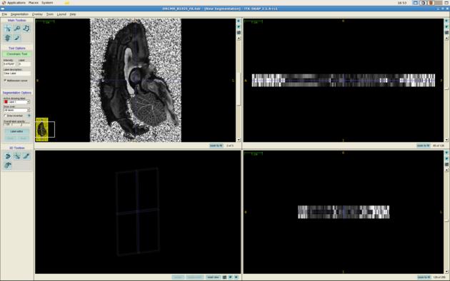
You can now view the images in an Analyze viewer of your choice. For example, here is a screen shot of DRCMR_B3091_FA.img viewed in itksnap:
itksnap DRCMR_B1925_FA.hdr
The command dtshape produces a range of other simple parameter maps derived from the diffusion tensor.
11. Visualize the RGB image with Matlab and pdview
Next, we'll compute the eigen system and extract some information from it.
dteig < DRCMR_B1925_DT.Bdouble > DRCMR_B1925_EIG.Bdouble
As before, we can see the RGB color-coded image using pdview, but we can also extract the information from the file for further processing. Each voxel in the output of dteig contains {l_1, e_11, e_12, e_13, l_2, e_21, e_22, e_33, l_3, e_31, e_32, e_33}, where l_1 >= l_2 >= l_3 and e_i = (e_i1, e_i2, e_i3) is the eigenvector with eigenvalue l_i.
Camino's shredder command is a useful tool for pulling out a subset of the values in each voxel of a data file. We can use it, for example, to extract the principal direction of the diffusion tensor from the output of dteig. The principal direction is elements 2, 3 and 4 of the twelve values per voxel output by dteig. The shredder command
shredder 8 24 72 < DRCMR_B1925_EIG.Bdouble > DRCMR_B1925_PD.Bdouble
skips the first 8 bytes of the input file (the first double, which is l_1 in the first voxel), then repeatedly outputs 24 bytes, skips 72 bytes, outputs 24 bytes, skips 72 bytes, until it reaches the end of the file. This outputs the next three doubles, ie e_11, e_12, e_13 in voxel one, and skips 9 doubles, taking us up to e_11, e_12, e_13 in voxel two, which shredder outputs, etc.
Now we can load this into MATLAB for processing. Here we'll simply generate the colour-coded direction map from DRCMR_B1925_PD.Bdouble:
% Load in the principal direction map.
fid = fopen('DRCMR_B1925_PD.Bdouble', 'r', 'b');
pd = fread(fid, 'double');
fclose(fid);
pd = reshape(pd, [3,128,256,3]);

% Load in the fractional anisotropy map
fid = fopen('DRCMR_B1925_FA.img', 'r', 'b');
fa = fread(fid, 'double');
fclose(fid);
fa = reshape(fa, [128,256,3]);

% Create the fa-weighted colour vector in each voxel
colfa = permute(abs(pd), [2 3 4 1]).*repmat(fa, [1 1 1 3]);

% Show slice 2
imshow(squeeze(colfa(:,:,2,:)))

% Write as png
imwrite(squeeze(colfa(:,:,2,:)), 'ColFA_Slice2.png', 'PNG');
Here is the image
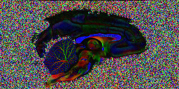
The colour encoding that appears for this data set is slightly unusual. By convention, red corresponds to left-right orientation, green to anterior-posterior and blue to inferior-superior. However, here, the corpus callosum, which has left-right orientation in the brain shows up blue. This is because the slice direction for this acquisition is along the left-right brain direction, ie slices are sagittal, rather than along the inferior-superior direction, giving axial slices, which is more common for human imaging. This can be fixed for display purposes by permuting the axes of the rgb
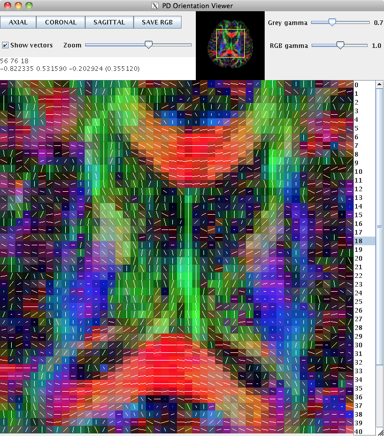
Looking at the image in pdview, we can see a more important problem, the principal direction vectors do not point along white matter fibres in the way they should. The vectors in the midsagittal corpus callosum correctly point out of the image plane as expects, but cingulate and cerebellar fibers have the wrong orientation.
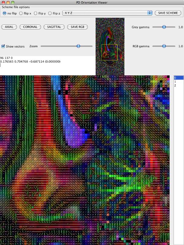
The problem here is a mismatch between the coordinate system of the image and that of the gradient directions used in the acquisition, ie those listed in the schemefile. The problem does not affect orientationally invariant indices derived from the diffusion tensor, like FA and MD. For procedures that rely on orientations, like tractography, we have to make the two coordinate systems match. pdview provides a mechanism for correcting the orientations in the schemefile to match the image if you specify the schemefile used in the DTI fitting:
pdview -scalarfile DRCMR_B1925_FA.hdr -schemefile DRCMR_B1925.scheme < DRCMR_B1925_EIG.Bdouble &
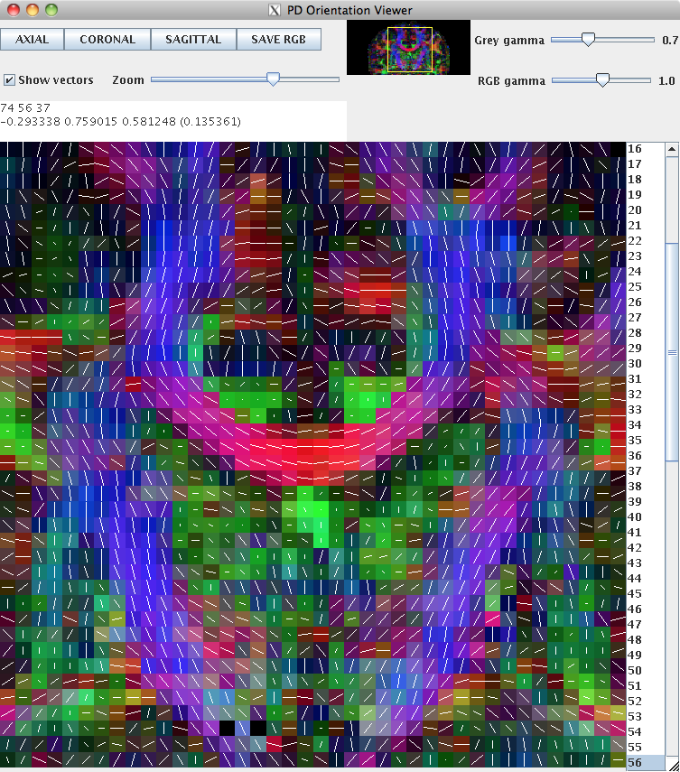
Note the extra panel in pdview listing scheme file options. You can figure out what permutation to make by thinking carefully about the image and gradient orientations, but often it is easier to do empirically once you know what you are looking for. Here, if we set the drop-down menu choice to "YXZ" instead of "XYZ" (specifying that the first and second schemefile coordinates are swapped compared to the image), which gives us
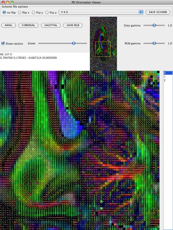
Now we need to save a version of the schemefile with the coordinate system corrected to match the image. Click the "Save Scheme" button and save it as DRCMR_B1925_Corr.scheme. Saving the scheme file does not alter the data, so we need to recompute the diffusion tensor with the corrected schemefile and recompute the eigensystem. We'll pipe the commands together to save disk space
dtfit DRCMR_B1925.Bfloat DRCMR_B1925_Corr.scheme | dteig | pdview -scalarfile DRCMR_B1925_FA.hdr