

On this page... (hide)
1. The VERDICT model for colorectal tumours
The tutorial demonstrates the VERDICT method- Vascular Extracellular and Restricted Diffusion for Cytometry in Tumours. The method is explained in detail in (Panagiotaki et al Cancer Research 2014, doi:10.1158/0008-5472.CAN-13-2511). Please cite that paper and the usual Camino ISMRM abstract if you use this.
The tutorial uses Camino to fit the VERDICT model to diffusion-weighted MRI data of tumour xenograft models of colorectal cancer and demonstrate microstructural parameter estimation.
This tutorial runs through an example of fitting the VERDICT colorectal model to a dataset from a human colorectal carcinoma cell line (LS174T), which you can get here LSDTIDWtut.Bfloat.zip. The file contains the normalised mean signal of all the voxels inside the tumour). Details about this dataset and the region of interest we select can be found in Panagiotaki et al. Cancer Research 2014 .
To follow this tutorial you need to have the following files:
- LSDTIDWtut.Bfloat
- VC_DTIDW.scheme
Schemefile: Requires STEJSKALTANNER. The scheme for the tumour dataset is VC_DTIDW.scheme.zip.
2. Fitting the VERDICT model
Here is an example for fitting the VERDICT colorectal model to the LS174T tumour data. The fitting assumes Gaussian noise.
ModelFit -inputfile LSDTIDWtut.Bfloat -inputdatatype float -fitmodel VERDICTcolorectal -fitalgorithm MULTIRUNLM -samples 100 -schemefile VC_DTIDW.scheme -noisemodel offgauss -sigma 0.0625 -voxels 1 -outputfile verd_LStut.Bfloat
The output file verd_LStut.Bfloat contains 100x12 values per voxel (for the 100 multiruns). They 12 values of the best run are:
- Exit code - indicating success/failure of the fitting procedure (0 means OK, -1 means background, anything else indicates a problem).
- S0 - the signal with no diffusion weighting.
- f1 - the vascular volume fraction (vascular compartment).
- f2 - the extra-cellular extravascular (EES) volume fraction (EES compartment).
- f3 - the intracellular volume fraction (intracellular compartment).
- P - the pseudo-diffusivity of water inside blood vessels in m^2/s.
- theta - angle of colatitude of the anisotropic tensor orientation.
- phi - angle of longitude of the anisotropic tensor orientation.
- d - the free diffusivity of the EES compartment in m^2/s.
- d - the diffusivity of the intracellular compartment in m^2/s.
- R - the axon radius index.
- fobj objective function
To see get the best run estimates you can use the following matlab code:
fid= fopen('verd_LStut.Bfloat','r','b');
d=fread(fid,'double');
fclose(fid);
d_sh= reshape(d,12,100);
[m,j]=min(d_sh(12,:))% get min fobj
d_sh(:,j) %to get the best parameters
Output:
- 0
- 1
- 0.1421
- 0.0805
- 0.7773
- 6.89E-09
- 1.0128
- 0.604464
- 9.00E-10
- 9.00E-10
- 7.9E-06
- 11.849
3. Plotting the fit of the VERDICT model to the scan data in Matlab
To plot the signal from the model you first need to generate synthetic data using the parameter estimates from the model fitting step. Here is the command for our example:
datasynth -synthmodel compartment 3 Stick 0.142 6.9e-9 1.012 0.604 Ball 0.08 9E-10 SPHEREGPD 9E-10 7.9e-6 -schemefile LSinvivo.scheme -voxels 1 -outputfile VC_lsSynth.Bfloat
The scheme for synthesizing data excluding the DTI dataset is VC_DW.scheme.zip. The file with the DW scan data is LSDWtut.Bfloat.zip.
For synthesizing data look at Synthesis using Analytic Models. Once you have your synthesized data you can load it onto Matlab and plot the signal using the following commands. For this you will need full_listColInv2.mat.zip.
To synthesize the signal for the model with the signal of the scan data run the following Matlab code:
%Load the list of imaging parameters (DELTA = gradient separation,
%delta = gradient duration, G = gradient strenth)
load full_listColInv2.mat;
%choose your Bfloat file  with the scan data LSDWtut.Bfloat
[FileName,PathName] = uigetfile('*.Bfloat','Select the bfloat-file');
fid=fopen(FileName,'r','b');
scanData= fread(fid,'float');
fclose(fid);

scanData = scanData';
%reshape the data
scanData= reshape(scanData,4, 43);
% b0 measurements
scan_b0 = scanData(1,:);
% fist direction
scan_dwpar = scanData(2,:);
% Second direction
scan_dwper1 = scanData(3,:);
% Third direction
scan_dwper2 = scanData(4,:);

%Find all the different values for DELTA
Delta_vec = unique(full_list(:, 1));
%Find the gradient strength
G = full_list(:, 3);

% Plot of scan data. The normalised signal S is
%plotted only for all the values of DELTA and delta as a function of the
%gradient strength |G| for all the directions.

for itDelta = 1:numel(Delta_vec)
Y=find(full_list(:,1)==Delta_vec(itDelta)& (full_list(:,2)<0.004));
d=find(full_list(:,1)==Delta_vec(itDelta)& (full_list(:,2)>0.004));
switch Delta_vec(itDelta)
case 0.01
char2='+';
case 0.02
char2='*';
case 0.03
char2='v';
case 0.04
char2='s';
case 0.05
char2='d';
end
hold on
plot(G(d),scan_dwper1(d),['c',char2],'MarkerSize',10,'LineWidth',1.5);
plot(G(Y),scan_dwper1(Y),['b',char2],'MarkerSize',10,'LineWidth',1.5);
plot(G(Y),scan_dwper2(Y),['g',char2],'MarkerSize',10,'LineWidth',1.5);
plot(G(d),scan_dwper2(d),['y',char2],'MarkerSize',10,'LineWidth',1.5);
plot(G(d),scan_dwpar(d),['k',char2],'MarkerSize',10,'LineWidth',1.5);
plot(G(Y),scan_dwpar(Y),['m',char2],'MarkerSize',10,'LineWidth',1.5);
title('Scan Data', 'FontSize', 14);
xlabel('G(T/m) ', 'FontSize', 14);
ylabel('S ', 'FontSize', 14);
end

hold on
load full_listColInv2.mat;
%choose your Bfloat file  with the synthesized data VC_lsSynth.Bfloat.
[FileName,PathName] = uigetfile('*.Bfloat','Select the bfloat-file');
fid=fopen(FileName,'r','b');
synthData= fread(fid,'float');
fclose(fid);

synthData = synthData';
%reshape the data
synthData= reshape(synthData,4, 43);
% b0 measurements
syn_b0 = synthData(1,:);
% first direction
syn_dwpar = synthData(2,:);
% Second direction
syn_dwper1 = synthData(3,:);
% Third direction
syn_dwper2 = synthData(4,:);


%Find all the different values for DELTA
Delta_vec = unique(full_list(:, 1));
%Find the gradient strength
G = full_list(:, 3);

% Plot of data synthesized from the model.
for itDelta = 1:numel(Delta_vec)
Y=find(full_list(:,1)==Delta_vec(itDelta)& (full_list(:,2)<0.004));
d=find(full_list(:,1)==Delta_vec(itDelta)& (full_list(:,2)>0.004));
switch Delta_vec(itDelta)
case 0.01
char2='-';
case 0.02
char2='-';
case 0.03
char2='-';
case 0.04
char2='-';
case 0.05
char2='-';
end
hold on
plot(G(d),syn_dwper1(d),['c',char2],'MarkerSize',10,'LineWidth',1.5);
plot(G(Y),syn_dwper1(Y),['b',char2],'MarkerSize',10,'LineWidth',1.5);
plot(G(Y),syn_dwper2(Y),['g',char2],'MarkerSize',10,'LineWidth',1.5);
plot(G(d),syn_dwper2(d),['y',char2],'MarkerSize',10,'LineWidth',1.5);
plot(G(d),syn_dwpar(d),['k',char2],'MarkerSize',10,'LineWidth',1.5);
plot(G(Y),syn_dwpar(Y),['m',char2],'MarkerSize',10,'LineWidth',1.5);
title('VERDICT', 'FontSize', 14);
xlabel('G(T/m) ', 'FontSize', 14);
ylabel('S ', 'FontSize', 14);
end
The resulting figure is below, which corresponds to Figure 1 in Panagiotaki et al. Cancer Research 2014.
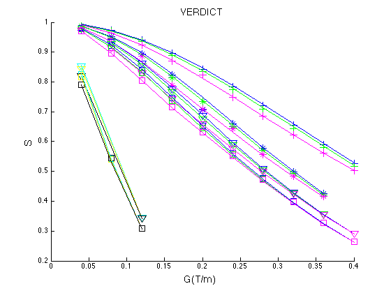
Figure 1. Fit of the VERDICT model to the DW data from the LS174T tumour. The symbols represent the measured data and the lines show the corresponding fits by the model. The normalized signal S is plotted for all values of delta and DELTA, as a function of the gradient strength |G|, for all diffusion directions (x, phase direction; y, read direction; z, slice direction).