
On this page... (hide)
1. White Matter Analytic Models
The tutorial uses Camino to fit analytic multi-compartment models to diffusion-weighted MRI data and demonstrate microstructural parameter estimation. The method is explained in detail in (Panagiotaki et al NeuroImage 2012, doi:10.1016/j.neuroimage.2011.09.081). Please cite that paper and the usual Camino ISMRM abstract if you use this.
This tutorial runs through an example of fitting two- and three-compartment models to a dataset which you can get here Data59meas.Bfloat.gz. This came from a fixed rat brain. The file contains the normalised mean signal of all the voxels with the fibre direction aligned with the central direction (direction aligned with the fibres in the corpus callosum and FA above a threshold). Figure 1 shows the imaging directions and Figure 2 shows a plot of the signal from the scan data. Details about this dataset and the region of interest we select can be found in Panagiotaki et al. NeuroImage 2012 .
To follow this tutorial you need to have the following files:
- Data59meas.Bfloat
- 59.scheme
Schemefile: Requires STEJSKALTANNER. The scheme for the fixed rat brain dataset is 59.scheme.gz.
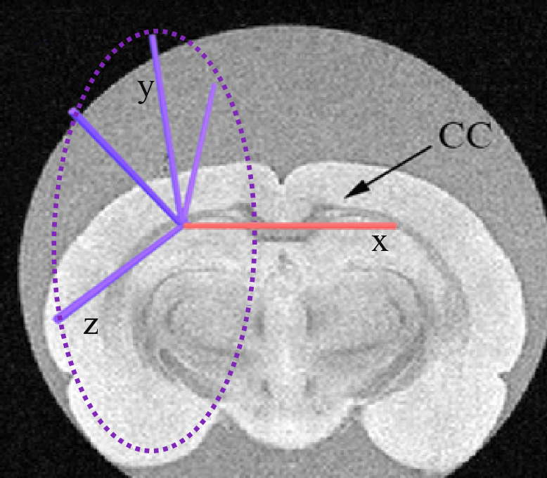
Figure 1. The red arrow indicates the central gradient direction used for the encoding scheme and the blue arrows indicate the four planar directions perpendicular to the central one
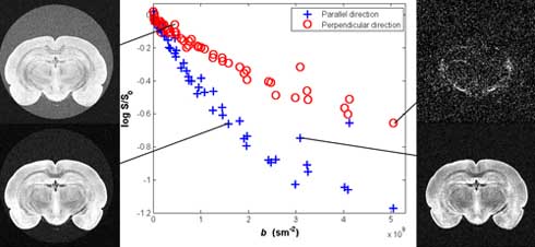
Figure 2. Plot of the parallel and the mean of the four perpendicular directions of the log signal from voxels in a region of interest in the corpus callosum and demonstration of MRI images for various b values
2. Plot the signal in Matlab
We can easily plot the signal using Matlab. For this you will need full_listFixedBrain.mat.gz.
%Load the list of imaging parameters (DELTA = gradient separation, delta = gradient duration, G = gradient strenth)
load full_listFixedBrain.mat;

%read the Bfloat file  with the scan data (Data59meas.Bfloat).
fid= fopen('Data59meas.Bfloat','r','b');
dw_data=fread(fid,'float');
fclose(fid);

dw_data= dw_data';
%reshape the data into the number of directions (5) and the number of
%measurements (59)
dw_data= reshape(dw_data,6, 59);
% b0 measurements
b0 = dw_data(1,:);
% parallel direction
dwpar = dw_data(2,:);
% First perpendicular direction
dwper1 = dw_data(3,:);
% Second perpendicular direction
dwper2 = dw_data(4,:);
% Third perpendicular direction
dwper3 = dw_data(5,:);
% Fourth perpendicular direction
dwper4 = dw_data(6,:);

%Take the mean of all the perpendicular directions
dwper =mean([dwper1;dwper2;dwper3;dwper4]);

% This step is required when the data is not normalised. In our example the data is normalised.
b0_norm = b0./b0;
dwpar_norm = dwpar./b0;
dwper_norm = dwper./b0;


%Find all the different values for DELTA
Delta_vec = unique(full_list(:, 1));
%Find the gradient strength
G = full_list(:, 3);

% Plot the normalised signal S for all the values of DELTA and delta as a function of the gradient strength |G| for the parallel and the perpendicular direction.

for itDelta = 1:numel(Delta_vec)
Y=find(full_list(:,1)==Delta_vec(itDelta)& (full_list(:,2)<0.004));
d=find(full_list(:,1)==Delta_vec(itDelta)& (full_list(:,2)>0.004));
switch Delta_vec(itDelta)
case 0.01
char2='+';
case 0.02
char2='*';
case 0.03
char2='v';
case 0.04
char2='s';
case 0.05
char2='d';
end
hold on
plot(G(d),dwper_norm(d),['k',char2],'MarkerSize',10,'LineWidth',1.5);
plot(G(d),dwpar_norm(d),['c',char2],'MarkerSize',10,'LineWidth',1.5);
plot(G(Y),dwper_norm(Y),['b',char2],'MarkerSize',10,'LineWidth',1.5);
plot(G(Y),dwpar_norm(Y),['m',char2],'MarkerSize',10,'LineWidth',1.5);
title('Scan Data', 'FontSize', 14);
xlabel('G(T/m) ', 'FontSize', 14);
ylabel('S ', 'FontSize', 14);
end
The resulting figure is this:
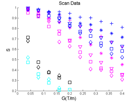
Figure 3. The normalised signal S is plotted for all the values of DELTA and delta as a function of the gradient strength |G| for the parallel and the mean of the four perpendicular directions.
3. Fitting the models
There are various options provided by Camino to fit an analytic model.
Modelfit options:
- fitmodel: selection of two- and three-compartment models (see list)
- fitalgorithm: LM, for using the Levenberg-Marquardt algorithm for a single run. MULTIRUNLM for multiple runs, using the optional flag "samples" to specify the number of multiruns (with a default of 100, otherwise).
- noisemodel: gaussian - for a fitting that assumes Gaussian noise, offgauss - assuming offset Gaussian noise; rician - assuming Rician noise. For the flags offgauss and rician you need to also define a "sigma". The sigma for the example dataset Data59meas.Bfloat is 0.0333.
- startpoint: allows you to define the starting values for the model (see example below).
Here is an example for a three-compartment model which assumes single radius cylinders for the intra-axonal space, cylindrical symmetry for the extra-axonal space and an isotropic restricted compartment with no radius and diffusivity (stationary water). The fitting assumes Gaussian noise.
modelfit -inputfile Data59meas.Bfloat -inputdatatype float -fitmodel ZEPPELINCYLINDERDOT -fitalgorithm LM -schemefile 59.scheme -voxels 1 -outputfile ZCD.Bdouble
The output file ZCD.Bdouble contains 14 values per voxel. They are:
- Exit code - indicating success/failure of the fitting procedure (0 means OK, -1 means background, anything else indicates a problem).
- S0 - the signal with no diffusion weighting.
- f1 - the intra-axonal volume fraction (restricted compartment).
- f2 - the extra-axonal white matter volume fraction (hindered compartment).
- f3 - the "stationary water" volume fraction.
- d - the intrinsic diffusivity of intra-axonal water in m^2/s.
- theta - angle of colatitude of axon orientation.
- phi - angle of longitude of axon orientation.
- R - the axon radius index.
- d - the parallel diffusivity of the hindered compartment in m^2/s.
- theta - angle of colatitude of principal direction of hindered diffusion (constrained equal to axon orientation).
- phi - angle of longitude of principal direction of hindered diffusion (constrained equal to axon orientation).
- d_perp - diffusivity of perpendicular hindered compartment
- fobj objective function
To see the outcome you use the following command:
cat ZCD.Bdouble | double2txt
Output:
- 0
- 0.996355083735763
- 0.344532605265831
- 0.331313540895689
- 0.324153853838481
- 8.28992411640961e-10
- 1.29330908738503
- -4.97044984292378
- 4.30378415135883e-06
- 8.28992411640961e-10
- 1.29330908738503
- -4.97044984292378
- 3.61562988020452e-10
- 0.324437715822494
To interpret the output of every multi-compartment model you can use the following guidelines. Here is the list with the order of model parameters appearing:
- Exit code,
- S0
- Intra-axonal volume fraction f1, which is always the f of the second name in the multi-compartment model, e.g. in ZeppelinCylinder f1 is the Cylinder's volume fraction
- Extra-axonal f2 is the f of the first name in the multi-compartment model, e.g. in the ZeppelinCylinder f2 is the Zeppelin's f
- Third compartment's f3, which is always the last name in the name of the multi-compartment model, e.g. ZeppelinCylinderSphere f3 is the Sphere's f.
Then we put in order the parameters of the intra-axonal compartment, then the parameters of the extra-axonal compartment and then the parameters of the isotropic restriction compartment. Last comes always the objective function.
The list with the parameters of the individual compartments can be found in the data synthesis tutorial here List of compartment models in Camino
Here is one more example for TensorStickAstrosticks: The parameters for each model are:
Tensor: d, theta, phi, d_perp1, d_perp2, alpha Stick: d, theta, phi Astrosticks: d
So the output for TensorStickAstrosticks will be:
- exit code
- S0
- f1: the Stick's f
- f2:the Tensor's f
- f3: the Astrostick's f
- d:of the Stick
- theta:of the Stick
- phi:of the Stick
- d: of the Tensor
- theta: of the Tensor
- phi: of the Tensor
- d_perp1:of the Tensor
- d_perp2: of the Tensor
- alpha: of the Tensor
- d: of the Astrosticks
- fobj
4. Using a starting point
In Camino, fits of a simple model are relatively independent of the starting position. More complex models are more sensitive to the starting position. Therefore, Camino uses by default parameter estimates of simpler models to provide initial estimates. For example, to get the starting point for the three-compartment TensorGDRCylindersSphere we use the estimate from the two-compartment TensorCylinder. In turn, the starting point for TensorCylinder uses fits from two simpler models: the BallCylinder and the TensorStick. The TensorStick starting point depends on the BallStick and the linear DT estimation. The BallCylinder depends on the BallStick. Finally the BallStick depends on the estimate of the linear DT estimation.
However, we can skip this step by introducing a specific starting point using the flag "startpoint", which would make the fitting procedure faster.
First you define how many compartments the model you want to fit has by adding "compartment" after the startpoint and the number of compartments next to it, then you define the intra-axonal model and its parameters, then the extra-axonal with its parameters and then the third compartment with its parameters.
Example:
modelfit -startpoint compartment 3 gammadistribradiicylinders 0.4 1.8 3E-6 6E-10 1.5 1.5 ZEPPELIN 0.2 6E-10 1.5 1.5 1E-10 Astrocylinders 6E-10 2E-6 -inputfile Data59meas.Bfloat -inputdatatype float -fitmodel ZEPPELINGDRCYLINDERSASTROCYLINDERS -fitalgorithm LM -schemefile 59.scheme -voxels 1 -outputfile ZGAc.Bfloat
This information is printed in your screen when you start the fitting: GAMMADISTRIBRADIICYLINDERS: vol frac= 0.4 params = 1.8 3.0E-6 6.0E-10 1.5 1.5 ZEPPELIN: vol frac= 0.2 params = 6.0E-10 1.5 1.5 1.0E-10 ASTROCYLINDERS: vol frac= 0.3999999999999999 params = 6.0E-10 2.0E-6
Note that you only have to define the intra-axonal volume fraction when you are fitting two-compartment models and the intra- and extra-axonal when you fit three compartment models. The last volume fraction is calculated from the other two.
Output:
- 0
- 1.05930353659862
- 0.322018937513680
- 0.000232257168341810
- 0.677748805317978
- 0.919271198509249
- 2.09045675597066e-06
- 8.60105740366949e-10
- 1.54364284117927
- 1.54295759945265
- 8.60105740366949e-10
- 1.54364284117927
- 1.54295759945265
- 3.21339719671925e-17
- 8.60105740366949e-10
- 1.92169668749291e-06
- 0.573595920976929
5. Avoiding local minimum
Camino also gives you the opportunity to choose the best fit parameters from the models after a number of perturbations of the starting parameters to ensure a good minimum. To perform multiple runs of the fitting we change the flag fitalgorithm to MULTIRUNLM for multiple runs, using the optional flag "samples" to specify the number of multiruns (with a default of 100, otherwise). Here is an example:
modelFit -inputfile Data59meas.Bfloat -inputdatatype float -fitmodel ZEPPELINCYLINDERDOT -fitalgorithm MULTIRUNLM -samples 1000 -schemefile 59.scheme -voxels 1 -noisemodel offGauss -sigma 0.0333 -outputfile ZCDmulti.Bfloat
The result of the MULTIRUN can help us evaluate the stability of the fit of the models. For example we can compute the histogram for the ZeppelinCylinderDot model of the final objective function obtained by the LM algorithm from each of the 1000 perturbations of the starting parameters. Here is the resulting figure, which corresponds to Figure 6 in the Panagiotaki et al NeuroImage 2012.
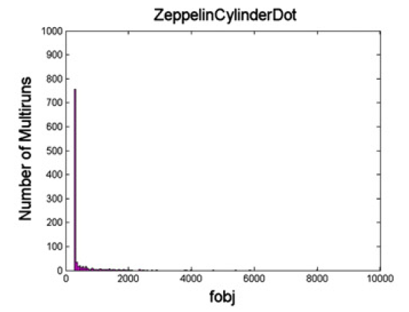
Figure 4. Histogram of the final objective function of 1000 runs for the ZeppelinCylinderDot model.
To quantify the difference among all the potential models more precisely we can estimate the number of runs required for each model to ensure obtaining the lowest objective function in at least one run with probability P>0.99. From the histograms we estimate the probability of finding the best solution in a single run as the fraction of the 1000 runs in the lowest histogram bin. The probability of not obtaining the best solution in N runs is then (1-pmodel)^N. To get the number of runs for P>0.99 we take the smallest integer N for which (1-pmodel)^N<0.01. For our example the ZeppelinCylinderDot model needs N=3 for P>0.99.
6. Plot the signal from the analytic model in Matlab
To plot the signal you first need to generate synthetic data with these models using the parameter estimates from the model fitting. Here is the command for our example :
datasynth -synthmodel compartment 3 CYLINDERGPD 0.345 8.289E-10 1.293 -4.97 4.3E-6 zeppelin 0.331 8.289E-9 1.293 -4.97 3.615E-10 Dot -schemefile 59.scheme -voxels 1 -outputfile ZCD.Bfloat
For synthesizing data look at Synthesis using Analytic Models. Once you have your synthesized data you can load it onto Matlab and plot the signal using the following commands. For this you will need full_listFixedBrain.mat.gz.
To synthesize the signal for the model with the signal of the scan data run the Matlab code as given in ( Plot the signal in Matlab) and add hold on. Then continue with the code below.
%Load the list of imaging parameters (DELTA = gradient separation, delta = gradient duration, G = gradient strenth)
load full_listFixedBrain.mat;
%choose your Bfloat file  with the synthesized data from ZCD.Bfloat.

fid= fopen('ZCD.Bfloat','r','b');
synthData=fread(fid,'float');
fclose(fid);

synthData = synthData';
%reshape the data into the number of directions (5) and the number of
%measurements (59)
synthData= reshape(synthData,6, 59);
% b0 measurements
syn_b0 = synthData(1,:);
% parallel direction
syn_dwpar = synthData(2,:);
% First perpendicular direction
syn_dwper1 = synthData(3,:);
% Second perpendicular direction
syn_dwper2 = synthData(4,:);
% Third perpendicular direction
syn_dwper3 = synthData(5,:);
% Fourth perpendicular direction
syn_dwper4 = synthData(6,:);

%Take the mean of all the perpendicular directions
syn_dwper =mean([syn_dwper1;syn_dwper2;syn_dwper3;syn_dwper4]);

%Normalise data
syn_b0_norm = syn_b0./syn_b0;
syn_dwpar_norm = syn_dwpar./syn_b0;
syn_dwper_norm = syn_dwper./syn_b0;


%Find all the different values for DELTA
Delta_vec = unique(full_list(:, 1));
%Find the gradient strength
G = full_list(:, 3);

% Plot of data synthesized from the model. The normalised signal S is
%plotted for all the values of DELTA and delta as a function of the
%gradient strength |G| for the parallel and the perpendicular direction.

for itDelta = 1:numel(Delta_vec)
Y=find(full_list(:,1)==Delta_vec(itDelta)& (full_list(:,2)<0.004));
d=find(full_list(:,1)==Delta_vec(itDelta)& (full_list(:,2)>0.004));
switch Delta_vec(itDelta)
case 0.01
char2='-';
case 0.02
char2='-';
case 0.03
char2='-';
case 0.04
char2='-';
case 0.05
char2='-';
end
hold on
plot(G(d),syn_dwper_norm(d),['k',char2],'MarkerSize',10,'LineWidth',1.5);
plot(G(d),syn_dwpar_norm(d),['c',char2],'MarkerSize',10,'LineWidth',1.5);
plot(G(Y),syn_dwper_norm(Y),['b',char2],'MarkerSize',10,'LineWidth',1.5);
plot(G(Y),syn_dwpar_norm(Y),['m',char2],'MarkerSize',10,'LineWidth',1.5);
title('Synthetic Data', 'FontSize', 14);
xlabel('G(T/m) ', 'FontSize', 14);
ylabel('S ', 'FontSize', 14);
end
The resulting figure is below, which corresponds to Figure 5 in Panagiotaki et al. NeuroImage 2012.
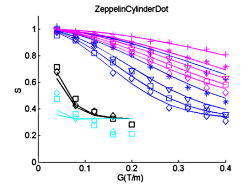
Figure 5. Synthesized data using the "ZeppelinCylinderDot" model.
7. List of analytic models in Camino
This is the full list of models used in Panagiotaki et al. NeuroImage 2012. You can run the whole procedure explained in this tutorial with all the models to replicate the results in the NeuroImage paper.
- DT
- Bizeppelin
- BallStick
- BallCylinder
- BallGDRCylinders
- ZeppelinStick
- ZeppelinCylinder
- ZeppelinGDRCylinders
- TensorStick
- TensorCylinder
- TensorGDRCylinders
- BallStickDot
- BallCylinderDot
- BallGDRCylindersDot
- ZeppelinStickDot
- ZeppelinCylinderDot
- ZeppelinGDRCylindersDot
- TensorStickDot
- TensorCylinderDot
- TensorGDRCylindersDot
- BallStickAstrosticks
- BallCylinderAstrosticks
- BallGDRCylindersAstrosticks
- ZeppelinStickAstrosticks
- ZeppelinCylinderAstrosticks
- ZeppelinGDRCylindersAstrosticks
- TensorStickAstrosticks
- TensorCylinderAstrosticks
- TensorGDRCylindersAstrosticks
- BallStickAstrocylinders
- BallCylinderAstrocylinders
- BallGDRCylindersAstrocylinders
- ZeppelinStickAstrocylinders
- ZeppelinCylinderAstrocylinders
- ZeppelinGDRCylindersAstrocylinders
- TensorStickAstrocylinders
- TensorCylinderAstrocylinders
- TensorGDRCylindersAstrocylinders
- BallStickSphere
- BallCylinderSphere
- BallGDRCylindersSphere
- ZeppelinStickSphere
- ZeppelinCylinderSphere
- ZeppelinGDRCylindersSphere
- TensorStickSphere
- TensorCylinderSphere
- TensorGDRCylindersSphere
8. Computing the BIC
We can use the Bayesian information criterion (BIC) (Schwarz, 1978) to evaluate the models. BIC chooses the most economical analytic model by rewarding those that minimise the objective function, while simultaneously penalising increasing numbers of model parameters:
BIC = -2ln(L) + kln(n),
where L is the likelihood of the estimated model, n is the number of measurements and k is the number of free model parameters to be estimated. The model which provides the lower value of the BIC is the one to be preferred.
9. Reference
-Eleftheria Panagiotaki, Torben Schneider, Bernard Siow, Matt G. Hall, Mark F. Lythgoe, Daniel C. Alexander Compartment models of the diffusion MR signal in brain white matter: A taxonomy and comparison NeuroImage 59 (4), 22412254,2012 (Panagiotaki et al. NeuroImage 2012 ).