Scheme files

Scheme files accompany DWI data and describe imaging parameters that are used in image processing. For most users, we require the gradient directions and b-value of each measurement in the sequence. Once you have this information, you can use the Camino commands described below to generate scheme files.

1.  Overview of scheme file formats

All Camino scheme files share some common characteristics:

• Plain text format. Numbers are specified in UK/US format, using periods for decimal points. Examples are: 1.0, -3.14, or 1.0E3.
• Comments are allowed, the line must start with #.
• The first non-comment line must be a header stating "VERSION: <version>".
• After removing comments and the header, measurements are described in order, one per line. The order must correspond to the order of the DWI data.
• Entries on each line are separated by spaces or tabs.

Particular scheme formats are described below:

1.1  BVECTOR

The BVECTOR is the most common scheme format. Each line consists of four values: the (x, y, z) components of the gradient direction followed by the b-value. For example:

   # Standard 6 DTI gradient directions, [b] = s / mm^2
  VERSION: BVECTOR
   0.000000   0.000000   0.000000   0.0
   0.707107   0.000000   0.707107   1.000E03
  -0.707107   0.000000   0.707107   1.000E03
   0.000000   0.707107   0.707107   1.000E03
   0.000000   0.707107  -0.707107   1.000E03
   0.707107   0.707107   0.000000   1.000E03
  -0.707107   0.707107   0.000000   1.000E03

If the measurement is unweighted, its gradient direction should be zero. Otherwise, the gradient directions should be unit vectors, followed by a scalar b-value.

The b-value can be in any units. Units are defined implicitly, in the above example we have used s / mm^2. The choice of units affects the scale of the output tensors, if we used this scheme file we would get tensors in units of mm^2 / s. We could change the units of b to s / m^2 by scaling the b-values by 1E6. Our reconstructed tensors would then be specified in units of m^2 / s.

There is no comprehensive standard for the choice of units. Different software will have different requirements. For some applications, such as computing fractional anisotropy, the units should be unimportant. Some applications, such as PICo tractography, require an awareness of units. In these cases the default expectation in Camino is standard units (meters, seconds, etc), unless you specify otherwise.

1.2  STEJSKALTANNER

This scheme format describes the standard Stejskal-Tanner pulse-gradient spin-echo pulse sequence. It has the following format:

VERSION: STEJSKALTANNER
x_1 y_1 z_1 |G_1| DELTA_1 delta_1 TE_1
x_2 y_2 z_2 |G_2| DELTA_2 delta_2 TE_2
:
:
x_N y_N z_N |G_N| DELTA_N delta_N TE_N

As before, the first line tells Camino what format to expect and each subsequent line represents one diffusion weighted image so that the (i+1)-th line represents the i-th diffusion weighted image. For the i-th image, (nx_i ny_i nz_i) is the gradient direction, |G_i| is the gradient strength, DELTA_i is the pulse separation (time between the onset of the first and second diffusion pulses), delta_i is the length of each pulse, TE_i is the echo time.

This format is essential for some more advanced operations in Camino, but for basic DTI the BVECTOR schemefile is fine and is independent of the specific pulse sequence. If you are not using the Stejskal-Tanner pulse sequence, for example Siemens machines use twice-refocussed pulse-sequence by default, it is best to stick with the simple BVECTOR schemefile above. A detailed schemefile format does actually exist for the twice refocussed sequence and a few other specific types.

Planning to add pictures of the pulse sequences here and the format of the TRSE schemefile

2.  Finding the information for the scheme file

The best way to find the information for your scheme file is to talk to the person who programmed your MRI sequence. There is software that can help you recover them from DICOM or other scanner-specific data formats. The dcm2nii program will attempt to recover b-values and vectors in FSL format.

3.  Converting to Camino format

If you have a list of gradient directions, you can convert them to Camino format by hand or by using pointset2scheme. If you have FSL style bval and bvec files, you can use fsl2scheme. See the man pages for more information.

4.  Checking results

Check for common problems with scheme definition. Some of these problems can be difficult to detect, some will affect tensor orientation but not tensor shape, so they may go undetected if you only look at FA or MD images.

4.1  Gradient orientation

Gradient orientations are often defined in magnet space, meaning that their orientation is defined relative to the magnet bore, and not relative to the field of view of the image. For axial images, this is usually a minor problem, because the image and magnet orientation either agree or can be brought into agreement by flipping the gradient axes in the scheme file.

You can preview the effect of a flip by loading your tensor eigen decomposition and scheme file into pdview. You need to check both an axial and a coronal slice.

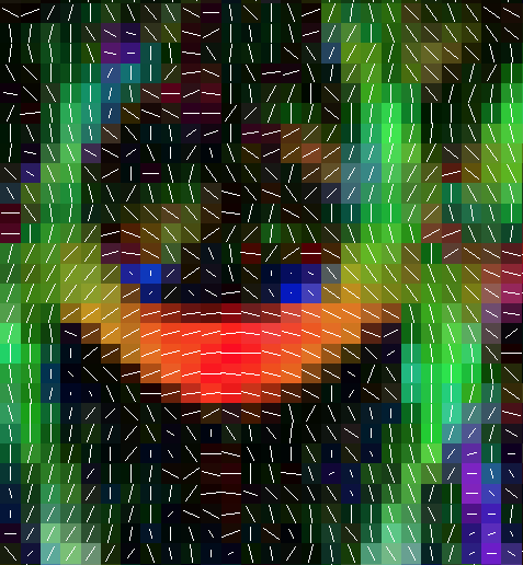
Axial slice of a reconstructed DT image. The x-coordinate of the principal direction is flipped.

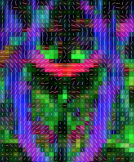
Coronal slice of a reconstructed DT image. The z-coordinate of the principal direction is flipped.

You can flip gradient directions in the scheme file interactively, until the principal directions look correct. You can also switch the ordering of the axes, for example if your images are acquired coronally rather than axially, then "z" in the voxel space will actually be "y" in the physical space. When you're done, you must save the scheme file and reconstruct your data - pdview will not modify your data, only the scheme file.

If the image orientation is unusual, for example if z is oblique to the magnet bore, you will need to rotate the gradient directions, or the tensors will be incorrectly aligned.

4.2  Measurements with zero diffusion weighting

Some scanners don't show the b=0 measurements in the gradient table. Usually this means that the b=0 volumes are acquired at the beginning of the scan. You can add zero measurements at the beginning of the scan in pointset2scheme. If the zero measurements are elsewhere, you will need to edit the scheme file by hand. Do this carefully because getting it wrong will alter the results in unpredictable ways.

4.3  Magnitude of gradient orientations can reflect different b-values

The b-value conventionally means the magnitude of diffusion sensitization built into the measurement. Some scanners allow the b-value to be adjusted on a per-measurement basis by changing the magnitude of the gradient directions from their usual unit value.

Typically, the diffusion weighted measurement is

where S₀ is the signal in the absence of diffusion weighting (b=0), r is a unit gradient direction, and b is the b-value. But if r can have arbitrary magnitude, then we don't know anything about the actual diffusion weighting unless we know both |r| and b for each measurement.

Some scanners will report a 'b-value' that applies to unit gradient directions, however the gradient table will include non-unit gradients. For example, imagine you are told b=1000 s / mm^2. The first measurement is r₁ =(1,0,0). But the next measurement is r₂ = (1, 1, 0). The magnitude of this second vector is sqrt(2), or 1.41. What this means is that the scanner applied both the x and the y gradients at full power, resulting in more diffusion weighting on the second measurement. Sometimes all gradient directions will have the same non-unit magnitude, in which case the b-value may or may not account for this.

Camino handles this by allowing you to optionally incorporate gradient magnitude into the b-value when you construct the scheme file. Thereafter, gradient directions in Camino are unit directions, and should remain so.