
NODDI Matlab Toolbox
What's New?
29th of Nov 2021: Introducing tissue-weighted mean to address a hitherto unrecognised bias with the conventional way of computing regional means in the presence of CSF partial volume. Links to full paper, 3-min summary, and code
12th of Jul 2021: A singularity container of NODDI toolbox has been made available by Dr Siya Sherif <s.sherif@uliege.be>
27th of Oct 2017: Check out our recent paper on validating NODDI with histological analysis, which was highlighted in a Nature Review article.
Introduction
This tutorial describes the fitting of NODDI data using Matlab. The tutorial includes the link to the NODDI matlab toolbox, an example NODDI data set, and a step-by-step instruction on how to use the toolbox to analyze the example data set.
Overview of NODDI
NODDI belongs to the family of diffusion MRI techniques underpinned by so-called multi-compartment models. Multi-compartment models interpret the MRI signals measured in each voxel as the sum of the contributions from the individual compartments that make up the voxel. This interpretation of the voxel-wise MRI signals confers the fundamental advantage of these models over the standard DTI, as well as the more recent diffusion kurtosis imaging (DKI). The metrics provided by DTI or DKI can only provide a composite view of the multifaceted contributions that may exist in a voxel. As a result, a change to DTI-drived FA may be caused by a host of underlying changes to the contributing compartments. In contrast, NODDI aims to disentangle the contribution from each compartment, thereby enabling their individualised characterisation. This distinction between DTI/DKI and NODDI is illustrated in Figure 1.
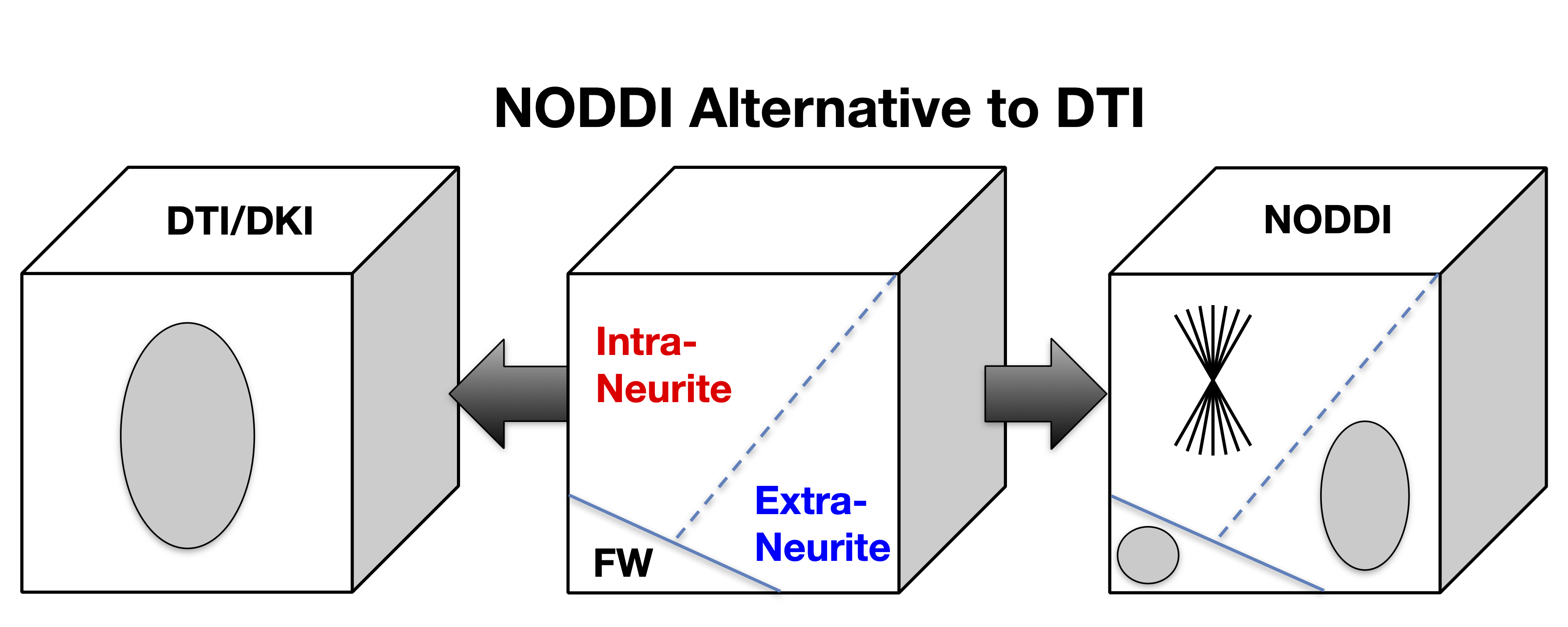 Figure 1: While DTI/DKI only provides a composite view of the complex neural tissue, NODDI offers an alternative that may enable the investigation of the contributing tissue components individually. (This work is licensed under a Creative Commons Attribution-NoDerivatives 4.0 International License).
NODDI enables the estimation of three key aspects of neural tissue at each voxel: neurite density index (NDI), which quantifies the packing density of axons or dendrites, orientation dispersion index (ODI), which assesses the orientation coherence of neurites, and the free water fraction (FWF), which estimates the extent of CSF contamination. Figure 2 illustrates the definition of these three key NODDI metrics and Figure 3 the spatial maps of these for the example dataset we provide in comparison to the standard DTI metrics (FA and MD).
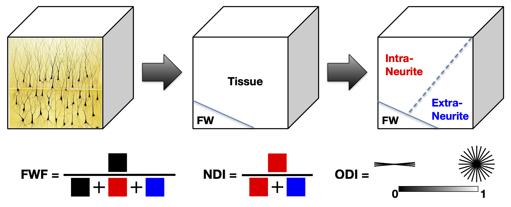 Figure 2: Definition of the three NODDI metrics illustrated schematically. (This work is licensed under a Creative Commons Attribution-NoDerivatives 4.0 International License).
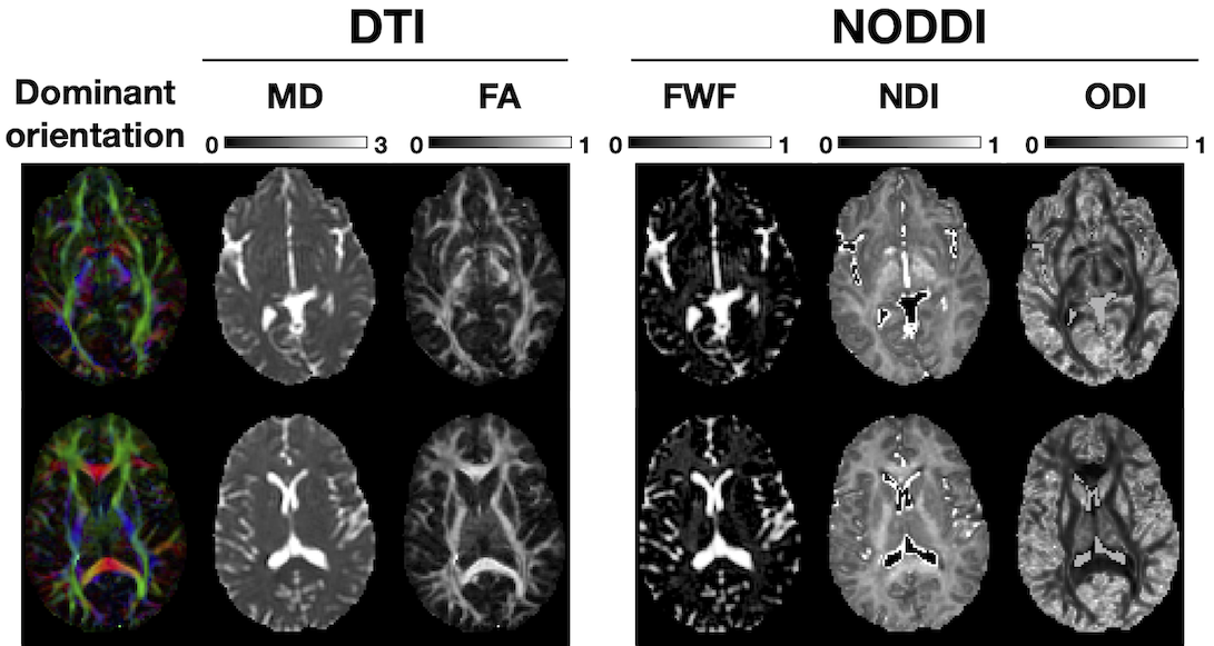 Figure 3: Example NODDI maps. (This work is licensed under a Creative Commons Attribution-NoDerivatives 4.0 International License).
If you need to learn more about NODDI, please refer to our NeuroImage paper or the video of the ISMRM 2012 presentation.
Applications of NODDI
For a list of recent applications of the NODDI technique, please visit the NODDI toolbox page on NITRC, which we use to host the software and example dataset downloads (see below).
Software requirements (Updated in October 2017)
The toolbox requires
- Matlab with the optimization toolbox
- NIFTI Matlab library: nifti_matlab
From the version 0.9 onward, the parallel computing Matlab toolbox will no longer be required but is recommended. See the instructions below for detail.
Download the toolbox
Click here to download the latest (July 2021) release: version 1.0.5. Please refer to the release notes for the detailed changes.
Download the example data set
The data set is available for download as a compressed zip archive.
The archive contains
- one 4-D diffusion-weighted MRI (DWI) volume:
NODDI_DWI.hdr/img - the corresponding brain region binary mask:
brain_mask.hdr/img - one region-of-interest (ROI) binary mask:
roi_mask.hdr/img - the corresponding NODDI protocol in FSL's bval/bvec format:
NODDI_protocol.bval/bvec - the expected outputs in the subdirectory
output(see below for the detail)
Acknowledgement: The example data set is generously provided by Dr. Gavin Winston from the UK Epilepsy Society MRI Unit at Chalfont. The MRI scanner at the unit is funded by the Big Lottery Fund, Wolfson Trust and the Epilepsy Society. The collection of this data was undertaken at UCLH/UCL who received a proportion of funding from the Department of Health's NIHR Biomedical Research Centres funding scheme.
Read the tutorial on how to explore DWI data (NEW)
I have written this tutorial after finding myself helping many users who have treated DWI data as a black box and never ventured to explore the data. Not doing so often prevents one to realise early on that there might be something wrong with the raw data, which could be either easily resolved issues concerning data formatting or organisation or more serious issues concerning the quality of the data.
This tutorial will help anyone develop a good understanding of how to look at DWI data and, in doing so, understand how the data should look like which will help identify issues with one's own data. It can be downloaded by clicking here.
Join NODDI google group
The NODDI google group keeps you up-to-date with the release of new versions with bug fixes and performance enhancement. It also provides a forum for you to send us your feedback and questions. So, please take a moment now to join the group by visiting http://groups.google.com/group/noddi.
Note that the forum is moderated: When you post a message for the first time, it will not appear automatically until we have a chance to verify that the message is not spam. So don't be alarmed if your message does not appear right away. The verification usually takes less than a day.
Step-by-step getting started tutorial
- Include nifti_matlab and NODDI toolbox in the matlab search path:
/usr/local/NODDI_tool, then run
addpath(genpath('/usr/local/NODDI_tool'))
rmpath(genpath('/usr/local/pkg/spm8'))
- Convert the raw DWI volume into the required format with the function
CreateROI:
/usr/local/NODDI_example_dataset, then to convert NODDI_DWI.hdr/img, first change your current directory to /usr/local/NODDI_example_dataset
cd /usr/local/NODDI_example_dataset
CreateROI('NODDI_DWI.hdr', 'roi_mask.hdr', 'NODDI_roi.mat');
- Convert the FSL bval/bvec files into the required format with the function
FSL2Protocol:
protocol = FSL2Protocol('NODDI_protocol.bval', 'NODDI_protocol.bvec');
For Camino users, the Scheme file can be converted into the required format with the function SchemeToProtocol:
protocol = SchemeToProtocol('NODDI_protocol.scheme');
- Create the NODDI model structure with the function
MakeModel:
noddi = MakeModel('WatsonSHStickTortIsoV_B0');
'WatsonSHStickTortIsoV_B0' is the internal name for the NODDI model. The structure noddi holds the details of the NODDI model relevant for the subsequent fitting. For most users, the default setting should suffice.
- Run the NODDI fitting with the function
batch_fitting, if you have the parallel computing toolbox, orbatch_fitting_single, if you do not:
batch_fitting('NODDI_roi.mat', protocol, noddi, 'FittedParams.mat', 8);
batch_fitting_single is similar:
batch_fitting_single('NODDI_roi.mat', protocol, noddi, 'FittedParams.mat');
batch_fitting, this function supports the resumption of an interrupted fitting run.(NEW)
- Convert the estimated NODDI parameters into volumetric parameter maps (Updated in May 2013):
SaveParamsAsNIfTI('FittedParams.mat', 'NODDI_roi.mat', 'brain_mask.hdr', 'example')
FittedParams.mat from an interrupted fitting run, from Version 1.04, the function will abort and will advise you to re-run the interrupted run.(NEW)
- Verify the output:
At this point, you should find the following output volumes:
- Neurite density (or intra-cellular volume fraction):
example_ficvf.nii - Orientation dispersion index (ODI):
example_odi.nii - CSF volume fraction:
example_fiso.nii - Fibre orientation:
example_fibredirs_{x,y,z}vec.nii - Fitting objective function values:
example_fmin.nii - Concentration parameter of Watson distribution used to compute ODI:
example_kappa.nii - Error code:
example_error_code.nii(NEW) Nonzero values indicate fitting errors.
- Neurite density (or intra-cellular volume fraction):
output subdirectory. (The content in the output directory will reflect the results from the pre-0.9 versions. So don't be alarmed if you do not see the error code volume.)
Questions or Comments
I hope you get to this point having successfully reproduced the step-by-step tutorial and are now ready to apply NODDI in your own studies. But if you do run into difficulties or have comments or suggestions, please don't hesitate to post them to the NODDI google group.